D'Agostino's K-squared test

In statistics, D’Agostino’s K² test is a goodness-of-fit measure of departure from normality, that is the test aims to establish whether or not the given sample comes from a normally distributed population. The test is based on transformations of the sample kurtosis and skewness, and has power only against the alternatives that the distribution is skewed and/or kurtic.

1 Skewness and kurtosis
2 Transformed sample skewness and kurtosis
3 Omnibus K² statistic
4 References

Skewness and kurtosis

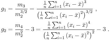
In the following, let { x_i } denote a sample of n observations, g₁ and g₂ are the sample skewness and kurtosis, m_j’s are the j-th sample central moments, and $\bar{x}$ is the sample mean. (Note that quite frequently in the literature related to normality testing the skewness and kurtosis are denoted as √β₁ and β₂ respectively. Such notation is less convenient since for example √β₁ can be a negative quantity).

The sample skewness and kurtosis are defined as

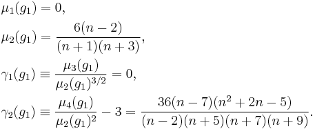
$\begin{align} & g_1 = \frac{ m_3 }{ m_2^{3/2} } = \frac{\frac{1}{n} \sum_{i=1}^n \left( x_i - \bar{x} \right)^3}{\left( \frac{1}{n} \sum_{i=1}^n \left( x_i - \bar{x} \right)^2 \right)^{3/2}}\ , \\ & g_2 = \frac{ m_4 }{ m_2^{2} }-3 = \frac{\frac{1}{n} \sum_{i=1}^n \left( x_i - \bar{x} \right)^4}{\left( \frac{1}{n} \sum_{i=1}^n \left( x_i - \bar{x} \right)^2 \right)^2} - 3\ . \end{align}$

These quantities consistently estimate the theoretical skewness and kurtosis of the distribution. Moreover, if the sample indeed comes from a normal population, then the exact finite sample distributions of the skewness and kurtosis can themselves be analysed in terms of their means μ₁, variances μ₂, skewnesses γ₁, and kurtoses γ₂. This has been done by Pearson (1931), who derived the following expressions:

$\begin{align} & \mu_1(g_1) = 0, \\ & \mu_2(g_1) = \frac{ 6(n-2) }{ (n%2B1)(n%2B3) }, \\ & \gamma_1(g_1) \equiv \frac{\mu_3(g_1)}{\mu_2(g_1)^{3/2}} = 0, \\ & \gamma_2(g_1) \equiv \frac{\mu_4(g_1)}{\mu_2(g_1)^{2}}-3 = \frac{ 36(n-7)(n^2%2B2n-5) }{ (n-2)(n%2B5)(n%2B7)(n%2B9) }. \end{align}$

and

$\begin{align} & \mu_1(g_2) = - \frac{6}{n%2B1}, \\ & \mu_2(g_2) = \frac{ 24n(n-2)(n-3) }{ (n%2B1)^2(n%2B3)(n%2B5) }, \\ & \gamma_1(g_2) \equiv \frac{\mu_3(g_2)}{\mu_2(g_2)^{3/2}} = \frac{6(n^2-5n%2B2)}{(n%2B7)(n%2B9)} \sqrt{\frac{6(n%2B3)(n%2B5)}{n(n-2)(n-3)}}, \\ & \gamma_2(g_2) \equiv \frac{\mu_4(g_2)}{\mu_2(g_2)^{2}}-3 = \frac{ 36(15n^6-36n^5-628n^4%2B982n^3%2B5777n^2-6402n%2B900) }{ n(n-3)(n-2)(n%2B7)(n%2B9)(n%2B11)(n%2B13) }. \end{align}$

For example, a sample with size n = 1000 drawn from a normally distributed population can be expected to have a skewness of 0 ± 0.08 and a kurtosis of 0 ± 0.15, where the ± indicates the standard deviation.

Transformed sample skewness and kurtosis

The sample skewness g₁ and kurtosis g₂ are both asymptotically normal. However the rate of their convergence to the distribution limit is frustratingly slow, especially for g₂. For example even with n = 5000 observations the sample kurtosis g₂ has both the skewness and the kurtosis of approximately 0.3, which is not negligible. In order to remedy this situation, it has been suggested to transform the quantities g₁ and g₂ in a way that makes their distribution as close to standard normal as possible.

In particular, D’Agostino (1970) suggested the following transformation for sample skewness:

$Z_1(g_1) = \delta\cdot \ln\!\left( \frac{g_1}{\alpha\sqrt{\mu_2}} %2B \sqrt{\frac{g_1^2}{\alpha^2\mu_2} %2B 1}\right),$

where constants α and δ are computed as

$\begin{align} & W^2 = \sqrt{2\gamma_2 %2B 4} - 1, \\ & \delta = 1 / \sqrt{\ln W}, \\ & \alpha^2 = 2 / (W^2-1), \\ \end{align}$

and where μ₂ = μ₂(g₁) is the variance of g₁, and γ₂ = γ₂(g₁) is the kurtosis — the expressions given in the previous section.

Similarly, Anscombe & Glynn (1983) suggested a transformation for g₂, which works reasonably well for sample sizes of 20 or greater:

$Z_2(g_2) = \sqrt{\frac{9A}{2}} \left\{1 - \frac{2}{9A} - \left(\frac{ 1-2/A }{ 1%2B\frac{g_2-\mu_1}{\sqrt{\mu_2}}\sqrt{2/(A-4)} }\right)^{\!1/3}\right\},$

where

$A = 6 %2B \frac{8}{\gamma_1} \left( \frac{2}{\gamma_1} %2B \sqrt{1%2B4/\gamma_1^2}\right),$

and μ₁ = μ₁(g₂), μ₂ = μ₂(g₂), γ₁ = γ₁(g₂) are the quantities computed by Pearson.

Omnibus K² statistic

Statistics Z₁ and Z₂ can be combined to produce an omnibus test, able to detect deviations from normality due to either skewness or kurtosis (D’Agostino, Belanger & D’Agostino 1990):

$K^2 = Z_1(g_1)^2 %2B Z_2(g_2)^2\,$

If the null hypothesis of normality is true, then K² is approximately χ²-distributed with 2 degrees of freedom.

Note that the statistics g₁, g₂ are not independent, only uncorrelated. Therefore their transforms Z₁, Z₂ will be dependent also (Shenton & Bowman 1977), rendering the validity of χ² approximation questionable. Simulations show that under the null hypothesis the K² test statistic is characterized by

	expected value	standard deviation	95% quantile
n = 20	1.971	2.339	6.373
n = 50	2.017	2.308	6.339
n = 100	2.026	2.267	6.271
n = 250	2.012	2.174	6.129
n = 500	2.009	2.113	6.063
n = 1000	2.000	2.062	6.038
χ²(2) distribution	2.000	2.000	5.991

References

Anscombe, F.J.; Glynn, William J. (1983). "Distribution of the kurtosis statistic b₂ for normal statistics". Biometrika 70 (1): 227–234. JSTOR 2335960.
D’Agostino, Ralph B. (1970). "Transformation to normality of the null distribution of g₁". Biometrika 57 (3): 679–681. JSTOR 2334794.
D’Agostino, Ralph B.; Albert Belanger; Ralph B. D’Agostino, Jr (1990). "A suggestion for using powerful and informative tests of normality". The American Statistician 44 (4): 316–321. JSTOR 2684359. http://www.cee.mtu.edu/~vgriffis/CE%205620%20materials/CE5620%20Reading/DAgostino%20et%20al%20-%20normaility%20tests.pdf.
Pearson, Egon S. (1931). "Note on tests for normality". Biometrika 22 (3/4): 423–424. JSTOR 2332104.
Shenton, L.R.; Bowman, K.O. (1977). "A bivariate model for the distribution of √b₁ and b₂". Journal of the American Statistical Association 72 (357): 206–211. JSTOR 2286939.

D'Agostino's K-squared test

Contents

Skewness and kurtosis

Transformed sample skewness and kurtosis

Omnibus K2 statistic

References

Omnibus K² statistic